Summarizing data with statistics, tables, and plots
foundations
In this Recipe we will explore appropriate methods for summarizing variables in datasets given the number and informational values of the variable(s). We will build on our understanding of how to summarize data using statistics, tables, and plots.
Skills
Summary overviews of datasets with {skimr}
Summary statistics with {dplyr}
Creating Quarto tables with {knitr}
Creating Quarto plots with {ggplot2}
Concepts and strategies
In this Recipe, we will use the PassiveBrownFam dataset from {corpora} (Evert 2023). This dataset contains information on the passive voice usage in the Brown family of corpora. The dataset contains 11 variables and 2,449 observations.
I have assigned this dataset to the object brown_fam_df and have made minor modifications to the variable names in Snippet 1 to improve the readability of the dataset.
Rows: 2,499
Columns: 11
$ id              <chr> "brown_A01", "brown_A02", "brown_A03", "brown_A04", "b…
$ corpus          <fct> Brown, Brown, Brown, Brown, Brown, Brown, Brown, Brown…
$ section         <fct> A, A, A, A, A, A, A, A, A, A, A, A, A, A, A, A, A, A, …
$ genre           <fct> press reportage, press reportage, press reportage, pre…
$ period          <fct> 1960, 1960, 1960, 1960, 1960, 1960, 1960, 1960, 1960, …
$ lang_variety    <fct> AmE, AmE, AmE, AmE, AmE, AmE, AmE, AmE, AmE, AmE, AmE,…
$ num_words       <int> 2080, 2116, 2051, 2095, 2111, 2102, 2099, 2069, 2058, …
$ active_verbs    <int> 164, 154, 135, 128, 170, 166, 165, 163, 153, 169, 132,…
$ passive_verbs   <int> 40, 25, 34, 25, 32, 21, 31, 19, 39, 23, 17, 10, 15, 26…
$ total_verbs     <int> 204, 179, 169, 153, 202, 187, 196, 182, 192, 192, 149,…
$ percent_passive <dbl> 19.61, 13.97, 20.12, 16.34, 15.84, 11.23, 15.82, 10.44…
You can learn more about these variables by reading the dataset documentation with ?corpora::PassiveBrownFam.
Statistical overviews
Understanding our data is of utmost importance before, during, and after analysis. After we get to know our data by inspecting the data origin, dictionary, and structure, we then move to summarizing the data.
A statistical overview of the data is a good place to start as it gives us a sense of all of the variables and variable types in the dataset. We can use {skimr} to create a statistical overview of the data, using the very convienent skim() function.
Let’s create a statistical overview of the brown_fam_df dataset in Snippet 2.
Snippet 2
# Load packageslibrary(skimr)# Create a statistical overview of the `brown_fam_df` datasetskim(brown_fam_df)
The output of the skim() function contains a lot of information but it essentially has two parts: a summary of the dataset and a summary of each variable in the dataset. The summary of each of the variables, however, is grouped by variable type. Remember, each of our variables in a data frame is a vector and each vector has a type.
We have already learned about different types of vectors in R, including character, numeric, and logical. In this dataset, we are presented with a new type of vector: a factor. A factor is essentially a character vector that contains a set of discrete values, or levels. Factors can be ordered or unordered and can contain levels that are not present in the data.
Now, looking at each of the variable types, we can see that we have 1 character variable, 5 factor variables, and 5 numeric variables. Each of these variable types assume a different set of summary statistics. For example, we can calculate the mean of a numeric variable but not of a character variable. Or, we can count the number of unique values in a character variable but not in a numeric variable.
For all variables, skim() will also provide the number of missing values and the percent of non-missing values.
Inspecting the entire dataset is a good place to start but at some point we often want focus in on a set of variables. We can add the yank() function to extract the statistical overview of a set of variables by their variable types.
Let’s extract the statistical overview of the numeric variables in the brown_fam_df dataset in Snippet 3.
Snippet 3
# Extract the statistical overview of the numeric variablesbrown_fam_df |>skim() |>yank("numeric")
These summary statistics are useful but for a preliminary and interactive use, but it is oftent the case that we will want to focus in on a particular variable or set of variables and their potential relationships to other variables.
We can use {dplyr} to calculate summary statistics for a particular variable or set of variables. We can use the group_by() function to group the data by a particular variable or variables. Then we can use the summarize() function to calculate summary statistics for the grouped data.
For example, let’s calculate the mean and median of the percent_passive variable in the brown_fam_df dataset grouped by the lang_variety variable, as seen in Snippet 4.
Snippet 4
# Mean and median of `percent_passive` grouped by `lang_variety`brown_fam_df |>group_by(lang_variety) |>summarize(mean_percent_passive =mean(percent_passive),median_percent_passive =median(percent_passive) )
The result is a 2x3 data frame which includes both the mean and median of the percent_passive variable for each of the two levels of the lang_variety variable.
The group_by() function can also be used to group by multiple variables. For example, in Snippet 5 we calculate the mean and median of the percent_passive variable in the brown_fam_df dataset grouped by the lang_variety and genre variables.
Snippet 5
# Mean and median of `percent_passive` grouped by# `lang_variety` and `genre`brown_fam_df |>group_by(lang_variety, genre) |>summarize(mean_percent_passive =mean(percent_passive),median_percent_passive =median(percent_passive) )
For numeric variables, such as percent_passive, there are a number of summary statistics that we can calculate. We’ve seen the R functions for mean and median but we can also calculate the standard deviation (sd()), variance (var()), minimum (min()), maximum (max()), interquartile range (IQR()), median absolute deviation (mad()), and quantiles (quantile()). All these calculations make sense for numeric variables but not for character variables.
For character variables, and factors, the summary statistics are more limited. We can calculate the number of observations (n()) and/ or the number of unique values (n_distinct()). Let’s now summarize the number of observations n() grouped by the genre variable in the brown_fam_df dataset in Snippet 6.
Snippet 6
# Frequency table for `genre`brown_fam_df |>group_by(genre) |>summarize(n =n(), )
Just as before, we can add multiple grouping variables to group_by(). Let’s add lang_variety to the grouping and calculate the number of observations n() grouped by the genre and lang_variety variables in the brown_fam_df dataset as seen in Snippet 7.
Snippet 7
# Cross-tabulation for `genre` and `lang_variety`brown_fam_df |>group_by(genre, lang_variety) |>summarize(n =n(), )
The result of calculating the number of observations for a character or factor variable is known as a frequency table. Grouping two or more categorical variables is known as a cross-tabulation or a contingency table.
Now, we can also pipe the results of a group_by() and summarize() to another function. This can be to say sort, select, or filter the results. It can also be to perform another summary function. It is important, however, to remember that the result of a group_by() produces a grouped data frame. Subsequent functions will be applied to the grouped data frame. This can lead to unexpected results if the original grouping is not relevant for the subsequent function. To avoid this, we can use the ungroup() function to remove the grouping after the relevant grouped summary statistics have been calculated.
Let’s return to calculating the number of observations n() grouped by the genre and lang_variety variables in the brown_fam_df dataset. But let’s add another summary which uses the n variable to calculate the mean and median number of observations.
If we do not use the ungroup() function, the mean and median will be calculated for each genre collapsed across lang_variety. We can see this in Snippet 8.
Snippet 8
# Mean and median of `n` grouped by `genre`brown_fam_df |>group_by(genre, lang_variety) |>summarize(n =n(), ) |>summarize(mean_n =mean(n),median_n =median(n) )
Therefore we see that we have a mean and median calculated for the number of documents in the corpus for each of the 15 genres.
If we use the ungroup() function, the mean and median will be calculated for all genres. Note we will use the ungroup() function between these summaries to clear the grouping before calculating the mean and median, as in Snippet 9.
Snippet 9
# Number of observations for each `genre` and `lang_variety`brown_fam_df |>group_by(genre, lang_variety) |>summarize(n =n(), ) |>ungroup() |>summarize(mean_n =mean(n),median_n =median(n) )
1
Use the ungroup() function to remove the grouping before calculating the mean and median.
Now we see that we have a mean and median calculated across all genres.
Before we leave this section, let’s look some other ways to create frequency and contingency tables for character and factor variables. A shortcut to calculate a frequency table for a character or factor variable is to use the count() function from {dplyr}.
Let’s calculate the number of observations grouped by the genre variable in the brown_fam_df dataset.
# Frequency table for `genre`brown_fam_df |>count(genre)
Note that the results of count() are not grouped so we do not need to use the ungroup() function before calculating subsequent summary statistics.
Another way to create frequency and contingency tables is to use the tabyl() function from {janitor} (Firke 2023). Let’s create a frequency table for the genre variable in the brown_fam_df dataset.
# Load packageslibrary(janitor)# Frequency table for `genre`brown_fam_df |>tabyl(genre)
In addition to providing frequency counts, the tabyl() function also provides the percent of observations for each level of the variable. And, we can add up to three grouping variables to tabyl() as well.
Let’s add lang_variety to the grouping and create a contingency table for the genre and lang_variety variables in the brown_fam_df dataset.
# Cross-tabulation for `genre` and `lang_variety`brown_fam_df |>tabyl(genre, lang_variety)
The results do not include the percent of observations for each level of the variable as it is not clear how to calculate the percent of observations for each level of the variable when there are multiple grouping variables. We must specify if we want to calculate the percent of observations by row or by column.
Dive deeper
{janitor} includes a variety of adorn_*() functions to add additional information to the results of tabyl(), including percentages, frequencies, and totals. Feel free to explore these functions on your own. We will return to this topic again later in the course.
Creating Quarto tables
Summarizing the data is not only useful for our understanding of the data as part of our analysis but also for communicating the data in reports, manuscripts, and presentations.
One way to communicate summary statistics is with tables. In Quarto, we can use {knitr} (Xie 2024) in combination with code block options to produce formatted tables which we can cross-reference in our prose sections.
Let’s create an object from the cross-tabulation for the genre and lang_variety variables in the brown_fam_df dataset to work with.
# Cross-tabulation for `genre` and `lang_variety`bf_genre_lang_ct <- brown_fam_df |>tabyl(genre, lang_variety)
To create a table in Quarto, we use the kable() function. The kable() function takes a data frame (or matrix) as an argument. The format argument will be derived from the Quarto document format (‘html’, ‘pdf’, etc.).
# Load packageslibrary(knitr)# Create a table in Quartokable(bf_genre_lang_ct)
            genre AmE BrE
  press reportage  88 132
  press editorial  54  81
    press reviews  34  51
         religion  34  51
 skills / hobbies  72 114
     popular lore  96 132
   belles lettres 150 231
    miscellaneous  60  90
          learned 160 240
  general fiction  58  87
        detective  48  72
  science fiction  12  18
        adventure  57  87
          romance  58  87
           humour  18  27
To add a caption to the table and to enable cross-referencing, we use the code block options label and tbl-cap. The label option takes a label prefixed with tbl- to create a cross-reference to the table. The tbl-cap option takes a caption for the table, in quotation marks.
#| label: tbl-brown-genre-lang-ct#| tbl-cap: "Cross-tabulation of `genre` and `lang_variety`"# Create a table in Quartokable(bf_genre_lang_ct)
Now we can cross-reference the table with the @tbl-brown-genre-lang-ct syntax. So the following Quarto document will produce the following prose with a cross-reference to the formatted table output.
As we see in @tbl-brown-genre-lang-ct, the distribution of `genre` is similar across `lang_variety`.```{r}#| label: tbl-brown-genre-lang-ct#| tbl-cap: "Cross-tabulation of `genre` and `lang_variety`"# Print cross-tabulationkable(bf_genre_lang_ct)```
As we see in Table 1, the distribution of genre is similar across lang_variety.
Table 1: Cross-tabulation of genre and lang_variety
genre
AmE
BrE
press reportage
88
132
press editorial
54
81
press reviews
34
51
religion
34
51
skills / hobbies
72
114
popular lore
96
132
belles lettres
150
231
miscellaneous
60
90
learned
160
240
general fiction
58
87
detective
48
72
science fiction
12
18
adventure
57
87
romance
58
87
humour
18
27
Dive deeper
{kableExtra} (Zhu 2024) provides additional functionality for formatting tables in Quarto.
Creating Quarto plots
Where tables are useful for communicating summary statistics for numeric and character variables, plots are useful for communicating relationships between variables especially when one or more of the variables is numeric. Furthermore, for complex relationships, plots can be more effective than tables.
In Quarto, we can use {ggplot2} (Wickham et al. 2024) in combination with code block options to produce formatted plots which we can cross-reference in our prose sections.
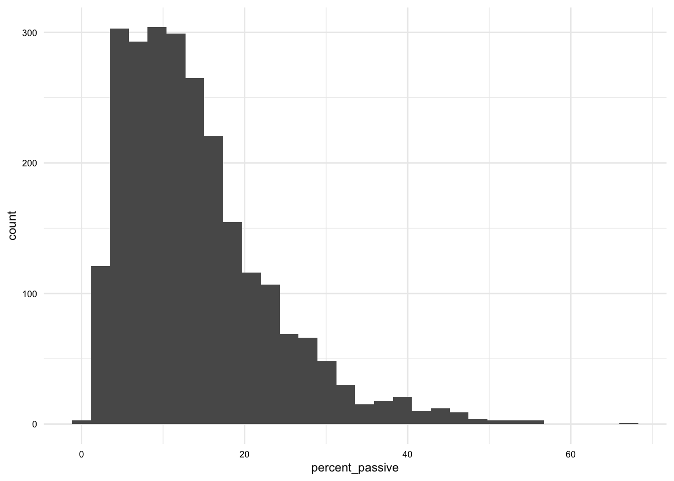
Let’s see this in action with a simple histogram of the percent_passive variable in the brown_fam_df dataset. The Quarto document will produce the following prose with a cross-reference to the formatted plot output.
As we see in @fig-brown-fam-percent-passive-hist, the distribution of `percent_passive` is skewed to the right.```{r}#| label: fig-brown-fam-percent-passive-hist#| fig-cap: "Histogram of `percent_passive`"# Create a histogram in Quartoggplot(brown_fam_df) + geom_histogram(aes(x = percent_passive))```
As we see in Figure 1, the distribution of percent_passive is skewed to the right.
Figure 1: Histogram of percent_passive
{ggplot2} implements the ‘Grammar of Graphics’ approach to creating plots. This approach is based on the idea that plots can be broken down into components, or layers, and that each layer can be manipulated independently.
The main components are data, aesthetics, and geometries. Data is the data frame that contains the variables to be plotted. Aesthetics are the variables that will be mapped to the x-axis, y-axis (as well as color, shape, size, etc.). Geometries are the visual elements that will be used to represent the data, such as points, lines, bars, etc..
As discussed in the R lesson “Visual Summaries”, the aes() function is used to map variables to aesthetics and can be added to the ggplot() function or to the geom_*() function depending on whether the aesthetic is mapped to all geometries or to a specific geometry, respectively.
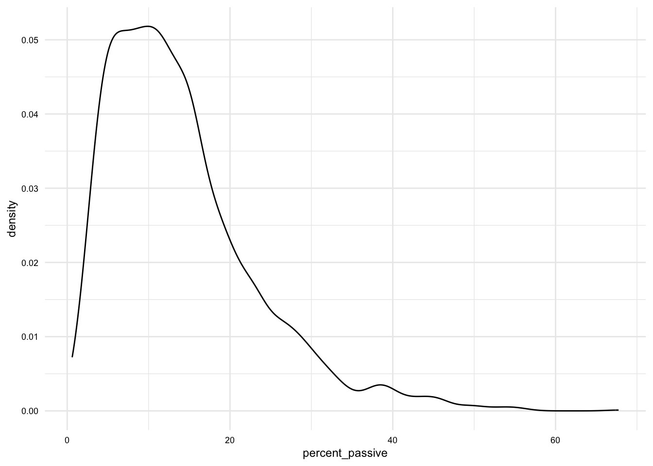
Take a look at the following stages of the earlier plot in each of the tabs below.
The geometries layer produces the plot connecting the data and aesthetics layers in the particular way specified by the geometries, in this case a histogram.
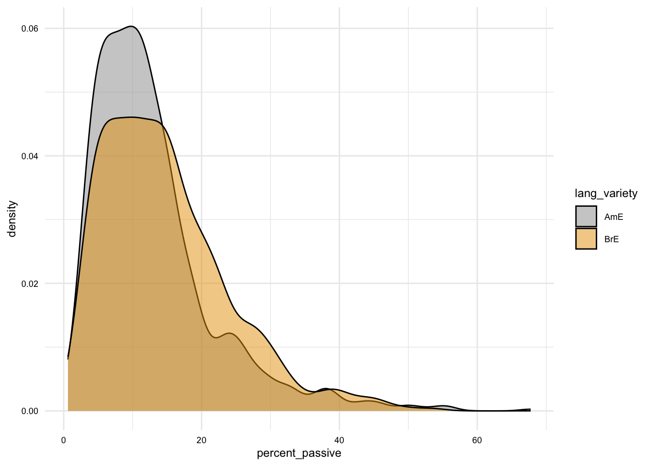
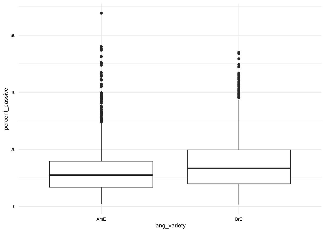
Just as with tables, the type of summary we choose to communicate with a plot depends on the type of variables we are working with and the relationships between those variables.
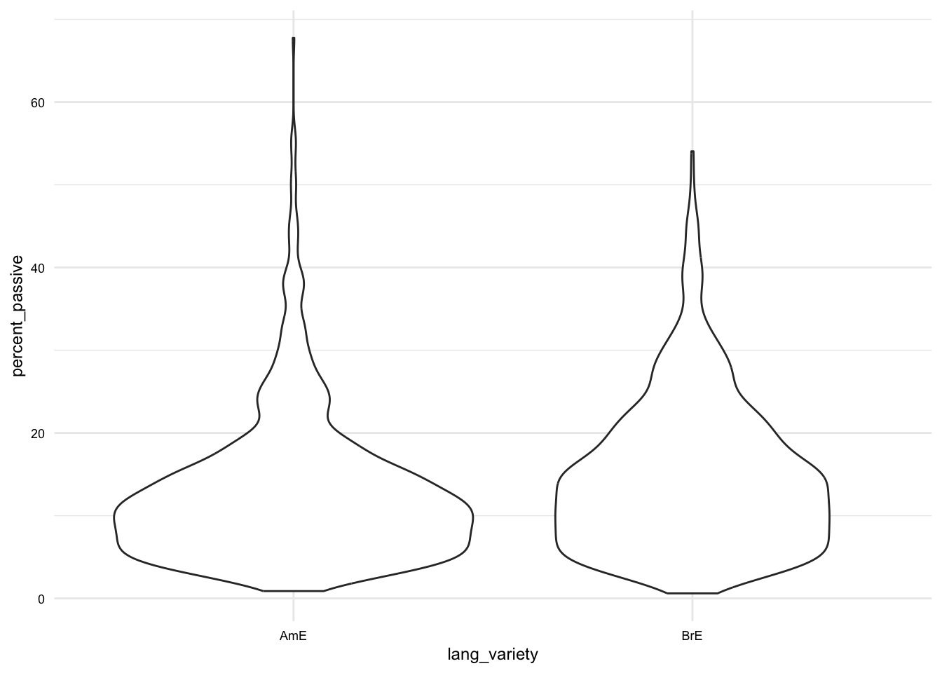
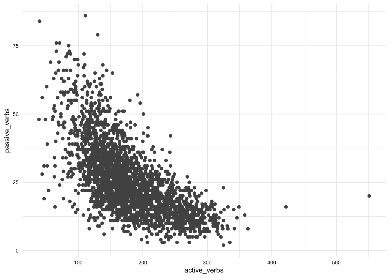
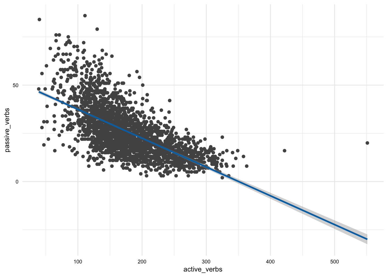
Below I’ve included a few examples of plots that can be used to communicate different types of variables and relationships.
In these examples, we have only looked at the most common variable combinations for one and two variable plots. There are more sophisticated plots that can be used for other variable combinations using {ggplot2}. For now, we will leave these for another time.
Check your understanding
A factor is a character vector augmented to include information about the discrete values, or levels, of the vector.
What is the difference between a frequency table and a contingency table?
The package is used to create formatted tables in R.
To add a geometry layer, such as geom_histogram(), to a ggplot object the |> operator is used.
To visualize the relationship between two numeric variables, a is often used.
When the aes() function is added to the ggplot() function, the aesthetic is mapped to all geometries.
Lab preparation
Before beginning Lab 03, learners should be comfortable with the skills and knowledge developed in the previous recipes and labs. In this lab, you will have a chance to use these skills and those introduced in this Recipe to provide a descriptive assessment of a dataset that includes statistics, tables, and plots using Quarto and R.
The additional skills and knowledge you will need to complete Lab 03 include:
Wickham, Hadley, Winston Chang, Lionel Henry, Thomas Lin Pedersen, Kohske Takahashi, Claus Wilke, Kara Woo, Hiroaki Yutani, Dewey Dunnington, and Teun van den Brand. 2024. Ggplot2: Create Elegant Data Visualisations Using the Grammar of Graphics. https://ggplot2.tidyverse.org.
Xie, Yihui. 2024. Knitr: A General-Purpose Package for Dynamic Report Generation in r. https://yihui.org/knitr/.