# Load packages
library(readr)
library(dplyr)
library(stringr)
library(purrr)
library(fs)
library(qtkit)06. Organizing and documenting data
Curating semi-structured data
preparation
After acquiring data, the next step in process is to organize data that is not tabular into a curated dataset. A curated dataset is a tidy dataset that reflects the data without major modifications. This dataset serves as a more general starting point for further data transformation. In this recipe, we will focus on curating data from a semi-structured format.
In this recipe, we will make use of {readr}, {dplyr}, {stringr}, and {purrr}, employ regular expressions to parse the semi-structured data, and use {qtkit} to document the dataset. Let’s load those packages now.
In Lab 6, we will apply what we learn in this recipe to curate and document acquired data.
Concepts and strategies
Assessing the data
Acquired data can be in a variety of formats. This will range from unstructured data such as running text to structured data such as tabular data. Semi-structured data is somewhere in between. It has some structure, but it is not as well defined as structured data and requires some work to organize it into a tidy dataset.
As a semi-structured example we will work with the The Switchboard Dialog Act Corpus (SWDA) (University of Colorado Boulder 2008) which extends the Switchboard Corpus with speech act annotation.
As a starting point, let’s assume you have acquired the SWDA corpus and decompressed it into your project’s data/original/swda/ directory, as seen below.
data/
├── analysis/
├── derived/
└── original/
    └── swda/
        ├── README
        ├── doc/
        ├── sw00utt/
        ├── sw01utt/
        ├── sw02utt/
        ├── sw03utt/
        ├── sw04utt/
        ├── sw05utt/
        ├── sw06utt/
        ├── sw07utt/
        ├── sw08utt/
        ├── sw09utt/
        ├── sw10utt/
        ├── sw11utt/
        ├── sw12utt/
        └── sw13utt/
The first step is to inspect the data directory and file structure (and of course any documentation files).
The README file contains basic information about the resource, the doc/ directory contains more detailed information about the dialog annotations, and each of the following directories prefixed with sw… contain individual conversation files.
Taking a closer look at the first conversation file directory, sw00utt/ we can see that it contains files with the .utt extension.
├── sw00utt
│   ├── sw_0001_4325.utt
│   ├── sw_0002_4330.utt
│   ├── sw_0003_4103.utt
│   ├── sw_0004_4327.utt
│   ├── sw_0005_4646.utt
Let’s take a look inside a conversation file (sw_0001_4325.utt) to see how it is structured internally. You can do this by opening the file in a text editor or by using the read_lines() function from the {readr} package.
*x*x*x*x*x*x*x*x*x*x*x*x*x*x*x*x*x*x*x*x*x*x*x*x*x*x*x*x*x*x*x*x*x*x*x*x*x*


FILENAME:   4325_1632_1519
TOPIC#:     323
DATE:       920323
TRANSCRIBER:    glp
UTT_CODER:  tc
DIFFICULTY: 1
TOPICALITY: 3
NATURALNESS:    2
ECHO_FROM_B:    1
ECHO_FROM_A:    4
STATIC_ON_A:    1
STATIC_ON_B:    1
BACKGROUND_A:   1
BACKGROUND_B:   2
REMARKS:        None.

=========================================================================


o          A.1 utt1: Okay.  /
qw          A.1 utt2: {D So, }

qy^d          B.2 utt1: [ [ I guess, +

+          A.3 utt1: What kind of experience [ do you, + do you ] have, then with child care? /

+          B.4 utt1: I think, ] + {F uh, } I wonder ] if that worked. /

qy          A.5 utt1: Does it say something? /

sd          B.6 utt1: I think it usually does.  /
There are few things to take note of here. First we see that the conversation files have a meta-data header offset from the conversation text by a line of = characters. Second, the header contains meta-information of various types. Third, the conversation text is interleaved with an annotation scheme.
Some of the information may be readily understandable, such as the various pieces of meta-data in the header, but to get a better understanding of what information is encoded here let’s take a look at the README file.
In this file we get a birds eye view of what is going on. In short, the data includes 1155 telephone conversations between two people annotated with 42 ‘DAMSL’ dialog act labels. The README file refers us to the doc/manual.august1.html file for more information on this scheme.
At this point we open the the doc/manual.august1.html file in a browser and do some investigation. We find out that ‘DAMSL’ stands for ‘Discourse Annotation and Markup System of Labeling’ and that the first characters of each line of the conversation text correspond to one or a combination of labels for each utterance. So for our first utterances we have:
o = "Other"
qw = "Wh-Question"
qy^d = "Declarative Yes-No-Question"
+ = "Segment (multi-utterance)"
Each utterance is also labeled for speaker (‘A’ or ‘B’), speaker turn (‘1’, ‘2’, ‘3’, etc.), and each utterance within that turn (‘utt1’, ‘utt2’, etc.). There is other annotation provided withing each utterance, but this should be enough to get us started on the conversations.
Now let’s turn to the meta-data in the header. We see here that there is information about the creation of the file: ‘FILENAME’, ‘TOPIC’, ‘DATE’, etc. The doc/manual.august1.html file doesn’t have much to say about this information so I returned to the LDC Documentation and found more information in the Online Documentation section. After some poking around in this documentation I discovered that that meta-data for each speaker in the corpus is found in the caller_tab.csv file. This tabular file does not contain column names, but the caller_doc.txt does. After inspecting these files manually and comparing them with the information in the conversation file I noticed that the ‘FILENAME’ information contained three pieces of useful information delimited by underscores _.
*x*x*x*x*x*x*x*x*x*x*x*x*x*x*x*x*x*x*x*x*x*x*x*x*x*x*x*x*x*x*x*x*x*x*x*x*x*


FILENAME:   4325_1632_1519
TOPIC#:     323
DATE:       920323
TRANSCRIBER:    glp
The first information is the document id (4325), the second and third correspond to the speaker number: the first being speaker A (1632) and the second speaker B (1519).
In sum, we have 1155 conversation files. Each file has two parts, a header and text section, separated by a line of = characters. The header section contains a ‘FILENAME’ line which has the document id, and ids for speaker A and speaker B. The text section is annotated with DAMSL tags beginning each line, followed by speaker, turn number, utterance number, and the utterance text. With this knowledge in hand, let’s set out to create a tidy dataset with the column structure as in Table 1.
| variable | name | type | description |
|---|---|---|---|
| doc_id | Document ID | character | The unique identifier for the conversation |
| damsl_tag | DAMSL Tag | character | The DAMSL tag for the utterance |
| speaker | Speaker | character | The speaker of the utterance |
| turn_num | Turn Number | character | The turn number of the utterance |
| utterance_num | Utterance Number | numeric | The utterance number of the utterance |
| utterance_text | Utterance Text | character | The text of the utterance |
| speaker_id | Speaker ID | character | The unique identifier for the speaker |
Tidy the data
There are many ways to approach the task of tidying the data in general, and this semi-structured data in particular. In this recipe, we will take a step-by-step approach to parsing the semi-structured data in one file and then apply this process to all of the files in the corpus using a custom function.
Let’s begin by reading one of the conversation files into R as a character vector using the read_lines() function from {readr}.
# Read a single file as character vector
doc_chr <-
  read_lines(file = "data/original/swda/sw00utt/sw_0001_4325.utt")
To isolate the vector element that contains the document and speaker ids, we use str_subset() from {stringr}. This function takes two arguments, a string and a pattern, and returns any vector element that matches the pattern.
In this case we are looking for a pattern that matches three groups of digits separated by underscores. To test out a pattern, we can use the str_view() function. We will use the regular expression character class \\d for digits and the + operator to match 1 or more contiguous digits. We then separate three groups of \\d+ with underscores _. The result is \\d+_\\d+_\\d+.
# Test out a pattern
doc_chr |>
  str_view(pattern = "\\d+_\\d+_\\d+")
[15] │ FILENAME:{\t}<4325_1632_1519>We can see that this pattern matches the line we are looking for. Now we can use this pattern with str_subset() to return the vector element that contains this pattern.
# Isolate the vector element that contains the document and speaker ids
str_subset(doc_chr, "\\d+_\\d+_\\d+")
[1] "FILENAME:\t4325_1632_1519"The next step is to extract the three digit sequences that correspond to the doc_id, speaker_a_id, and speaker_b_id. First we extract the pattern that we have identified with str_extract() and then we can break up the single character vector into multiple parts based on the underscore _. The str_split() function takes a string and then a pattern to use to split a character vector. It will return a list of character vectors.
str_subset(doc_chr, "\\d+_\\d+_\\d+") |> # isolate vector element
  str_extract("\\d+_\\d+_\\d+") |> # extract the pattern
  str_split("_") # split the character vector by underscore
[[1]]
[1] "4325" "1632" "1519"A list is a special object type in R. It is an unordered collection of objects whose lengths can differ (contrast this with a data frame which is a collection of objects whose lengths are the same –hence the tabular format).
In this case we have a list of length 1, whose sole element is a character vector of length 3 –one element per segment returned from our split. This is a desired result in most cases as if we were to pass multiple character vectors to our str_split() function we don’t want the results to be conflated as a single character vector blurring the distinction between the individual character vectors.
In this case, however, we want to extract the three elements of the character vector and assign them to meaningful variable names. To do this we will use the unlist() function which will convert the list into a single character vector. We will assign this result to speaker_info_chr.
speaker_info_chr <-
  str_subset(doc_chr, "\\d+_\\d+_\\d+") |>
  str_extract("\\d+_\\d+_\\d+") |>
  str_split("_") |>
  unlist() # convert the list to a character vector

# Preview
speaker_info_chr
[1] "4325" "1632" "1519"speaker_info_chr is now a character vector of length three. Let’s subset each of the elements and assign them to meaningful variable names so we can conveniently use them later on in the tidying process.
doc_id <- speaker_info_chr[1] # extract by index
speaker_a_id <- speaker_info_chr[2] # extract by index
speaker_b_id <- speaker_info_chr[3] # extract by index
The next step is to isolate the text section extracting it from rest of the document. As noted previously, a sequence of = separates the header section from the text section. What we need to do is to index the point in our character vector doc_chr where that line occurs and then subset the doc_chr from that point until the end of the character vector.
Let’s first find the point where the = sequence occurs. We will again use the str_view() to test out a pattern that matches a contiguous sequence of =.
str_view(doc_chr, "=+")[31] │ <=========================================================================>So for this file we see there is one element that matches and that element’s index is 31.
Now it is important to keep in mind that we are working with a single file from the swda/ data. Since our plan is to use this code to apply to other files, we need to be cautious to not create a pattern that may be matched multiple times in another document in the corpus. As the =+ pattern will match =, or ==, or ===, etc. it is not implausible to believe that there might be a = character on some other line in one of the other files.
Let’s update our regular expression to avoid this potential scenario by only matching sequences of three or more =. In this case we will make use of the curly bracket operators {}.
str_view(doc_chr, "={3,}")[31] │ <=========================================================================>We will get the same result for this file, but will safeguard ourselves a bit as it is unlikely we will find multiple matches for ===, ====, etc.
To extract just the index of the match, we can use the str_which() function with the same pattern. This will return the index of the vector element that matches the pattern. However, consider what we are doing. We actually are using this index to subset the vector, so we need to increment the index by 1 to get the next vector element. Let’s do this and then assign the result to text_start_index.
# Find where text starts
text_start_index <- str_which(doc_chr, "={3,}") + 1
The index for the end of the text is simply the length of the doc_chr vector. We can use the length() function to get this index.
# Find where text ends
text_end_index <- length(doc_chr)
We now have the bookends, so to speak, for our text section. To extract the text we subset the doc_chr vector by these indices.
# Extract text between indices
text <- doc_chr[text_start_index:text_end_index]

# Preview
head(text)
[1] " "
[2] ""
[3] "o A.1 utt1: Okay. /"
[4] "qw A.1 utt2: {D So, } "
[5] ""
[6] "qy^d B.2 utt1: [ [ I guess, + "The text has some extra whitespace on some lines and there are blank lines as well. We should do some cleaning up before moving forward to organize the data. To get rid of the whitespace we use the str_trim() function which by default will remove leading and trailing whitespace from each line.
# Remove leading and trailing whitespace
text <- str_trim(text)

# Preview
head(text)
[1] ""
[2] ""
[3] "o A.1 utt1: Okay. /"
[4] "qw A.1 utt2: {D So, }"
[5] ""
[6] "qy^d B.2 utt1: [ [ I guess, +"To remove blank lines we will use str_subset() to subset the text vector. The .+ pattern will match elements that are not blank. We will assign the result to text overwriting the original text vector.
# Remove blank lines
text <- str_subset(text, ".+")

# Preview
head(text)
[1] "o A.1 utt1: Okay. /"
[2] "qw A.1 utt2: {D So, }"
[3] "qy^d B.2 utt1: [ [ I guess, +"
[4] "+ A.3 utt1: What kind of experience [ do you, + do you ] have, then with child care? /"
[5] "+ B.4 utt1: I think, ] + {F uh, } I wonder ] if that worked. /"
[6] "qy A.5 utt1: Does it say something? /" Our first step towards a tidy dataset is to now combine the doc_id and each element of text in a data frame, leaving aside our speaker ids. We will use the tibble() function and pass the variables as named arguments.
# Combine info and text into a data frame
swda_df <- tibble(doc_id, text)

# Preview
slice_head(swda_df, n = 5)
# A tibble: 5 × 2
doc_id text
<chr> <chr>
1 4325 o A.1 utt1: Okay. /
2 4325 qw A.1 utt2: {D So, }
3 4325 qy^d B.2 utt1: [ [ I guess, +
4 4325 + A.3 utt1: What kind of experience [ do you, + do you ] have…
5 4325 + B.4 utt1: I think, ] + {F uh, } I wonder ] if that worked. /With our data now in a data frame, it’s time to parse the text column and extract the damsl tags, speaker, speaker turn, utterance number, and the utterance text itself into separate columns.
To do this we will make extensive use of regular expressions. Our aim is to find a consistent pattern that distinguishes each piece of information from other other text in a given row.
The best way to learn regular expressions is to use them. To this end I’ve included a link to the interactive regular expression practice website regex101.
Open this site and copy the text below into the ‘TEST STRING’ field.
o          A.1 utt1: Okay.  /
qw          A.1 utt2: {D So, }
qy^d          B.2 utt1: [ [ I guess, +
+          A.3 utt1: What kind of experience [ do you, + do you ] have, then with child care? /
+          B.4 utt1: I think, ] + {F uh, } I wonder ] if that worked. /
qy          A.5 utt1: Does it say something? /
sd          B.6 utt1: I think it usually does.  /
ad          B.6 utt2: You might try, {F uh, }  /
h          B.6 utt3: I don't know,  /
ad          B.6 utt4: hold it down a little longer,  /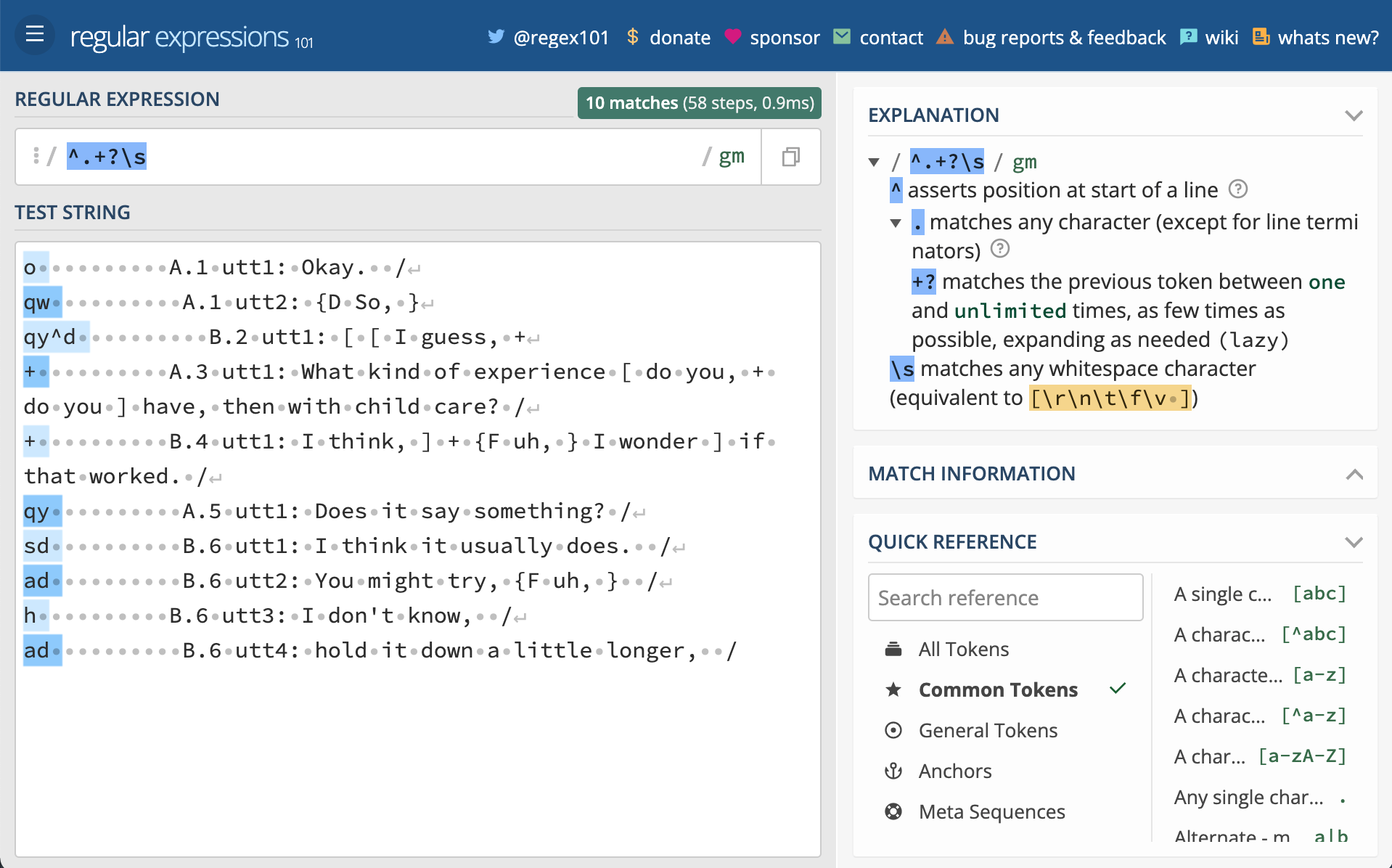
Now manually type the following regular expressions into the ‘REGULAR EXPRESSION’ field one-by-one (each is on a separate line). Notice what is matched as you type and when you’ve finished typing. You can find out exactly what the component parts of each expression are doing by toggling the top right icon in the window or hovering your mouse over the relevant parts of the expression.
^.+?\s
[AB]\.\d+
utt\d+
:.+$
As you can now see, we have regular expressions that will match the damsl tags, speaker and speaker turn, utterance number, and the utterance text.
To apply these expressions to our data and extract this information into separate columns we will make use of the mutate() and str_extract() functions. mutate() will take our data frame and create new columns with values we match and extract from each row in the data frame with str_extract().
I’ve chained each of these steps in the code below, dropping the original text column with select(-text), and overwriting swda_df with the results.
# Extract column information from `text`
swda_df <-
  swda_df |> # current dataset
  mutate(damsl_tag = str_extract(text, "^.+?\\s")) |> # damsl tags
  mutate(speaker_turn = str_extract(text, "[AB]\\.\\d+")) |> # speaker_turn pairs
  mutate(utterance_num = str_extract(text, "utt\\d+")) |> # utterance number
  mutate(utterance_text = str_extract(text, ":.+$")) |> # utterance text
  select(-text) # drop the `text` column

# Preview
glimpse(swda_df)
Rows: 159
Columns: 5
$ doc_id <chr> "4325", "4325", "4325", "4325", "4325", "4325", "4325",…
$ damsl_tag <chr> "o ", "qw ", "qy^d ", "+ ", "+ ", "qy ", "sd ", "ad ", …
$ speaker_turn <chr> "A.1", "A.1", "B.2", "A.3", "B.4", "A.5", "B.6", "B.6",…
$ utterance_num <chr> "utt1", "utt2", "utt1", "utt1", "utt1", "utt1", "utt1",…
$ utterance_text <chr> ": Okay. /", ": {D So, }", ": [ [ I guess, +", ": What…There are a couple things left to do to the columns we extracted from the text before we move on to finishing up our tidy dataset. First, we need to separate the speaker_turn column into speaker and turn_num columns and second we need to remove unwanted characters from the damsl_tag, utterance_num, and utterance_text columns.
To separate the values of a column into two columns we use the separate_wider_delim() function. It takes a column to separate, a delimiter to use to separate the values, and a character vector of the names of the new columns to create.
# Separate speaker_turn into distinct columns
swda_df <-
  swda_df |>
  separate_wider_delim(
    cols = speaker_turn,
    delim = ".",
    names = c("speaker", "turn_num")
  )

# Preview
glimpse(swda_df)
Rows: 159
Columns: 6
$ doc_id <chr> "4325", "4325", "4325", "4325", "4325", "4325", "4325",…
$ damsl_tag <chr> "o ", "qw ", "qy^d ", "+ ", "+ ", "qy ", "sd ", "ad ", …
$ speaker <chr> "A", "A", "B", "A", "B", "A", "B", "B", "B", "B", "B", …
$ turn_num <chr> "1", "1", "2", "3", "4", "5", "6", "6", "6", "6", "6", …
$ utterance_num <chr> "utt1", "utt2", "utt1", "utt1", "utt1", "utt1", "utt1",…
$ utterance_text <chr> ": Okay. /", ": {D So, }", ": [ [ I guess, +", ": What…To remove unwanted leading or trailing whitespace we apply the str_trim() function. For removing other characters we matching the character(s) and replace them with an empty string ("") with the str_replace() function. Again, I’ve chained these functions together and overwritten data with the results.
# Clean up column information
swda_df <-
  swda_df |> # current dataset
  mutate(damsl_tag = str_trim(damsl_tag)) |> # remove leading/ trailing whitespace
  mutate(utterance_num = str_replace(utterance_num, "utt", "")) |> # remove 'utt'
  mutate(utterance_text = str_replace(utterance_text, ":\\s", "")) |> # remove ': '
  mutate(utterance_text = str_trim(utterance_text)) # trim leading/ trailing whitespace

# Preview
glimpse(swda_df)
Rows: 159
Columns: 6
$ doc_id <chr> "4325", "4325", "4325", "4325", "4325", "4325", "4325",…
$ damsl_tag <chr> "o", "qw", "qy^d", "+", "+", "qy", "sd", "ad", "h", "ad…
$ speaker <chr> "A", "A", "B", "A", "B", "A", "B", "B", "B", "B", "B", …
$ turn_num <chr> "1", "1", "2", "3", "4", "5", "6", "6", "6", "6", "6", …
$ utterance_num <chr> "1", "2", "1", "1", "1", "1", "1", "2", "3", "4", "5", …
$ utterance_text <chr> "Okay. /", "{D So, }", "[ [ I guess, +", "What kind of…To round out our tidy dataset for this single conversation file we will connect the speaker_a_id and speaker_b_id with speaker A and B in our current dataset adding a new column speaker_id. The case_when() function does exactly this: allows us to map rows of speaker with the value “A” to speaker_a_id and rows with value “B” to speaker_b_id.
# Link speaker with speaker_id
swda_df <-
  swda_df |> # current dataset
  mutate(speaker_id = case_when( # create speaker_id
    speaker == "A" ~ speaker_a_id, # speaker_a_id value when A
    speaker == "B" ~ speaker_b_id, # speaker_b_id value when B
    TRUE ~ NA_character_ # NA otherwise
  ))

# Preview
glimpse(swda_df)
Rows: 159
Columns: 7
$ doc_id <chr> "4325", "4325", "4325", "4325", "4325", "4325", "4325",…
$ damsl_tag <chr> "o", "qw", "qy^d", "+", "+", "qy", "sd", "ad", "h", "ad…
$ speaker <chr> "A", "A", "B", "A", "B", "A", "B", "B", "B", "B", "B", …
$ turn_num <chr> "1", "1", "2", "3", "4", "5", "6", "6", "6", "6", "6", …
$ utterance_num <chr> "1", "2", "1", "1", "1", "1", "1", "2", "3", "4", "5", …
$ utterance_text <chr> "Okay. /", "{D So, }", "[ [ I guess, +", "What kind of…
$ speaker_id <chr> "1632", "1632", "1519", "1632", "1519", "1632", "1519",…We now have the tidy dataset we set out to create. But this dataset only includes one conversation file! We want to apply this code to all 1,155 conversation files in the swda/ corpus.
The approach will be to create a custom function which groups the code we’ve done for this single file and then iteratively send each file from the corpus through this function and combine the results into one data frame.
Here’s the custom function with some extra code to print a progress message for each file when it runs.
# [ ] add to {qtkit}, note the convention of `extract_` prefix for curation functions. In combination with `get_archive_data()` this corpus can be curated with few steps.

curate_swda_data <- function(file) {
  # Progress message
  file_basename <- basename(file) # file name
  message("Processing ", file_basename, "\n")

  # Read `file` by lines
  doc_chr <- read_lines(file)

  # Extract `doc_id`, `speaker_a_id`, and `speaker_b_id`
  speaker_info_chr <-
    str_subset(doc_chr, "\\d+_\\d+_\\d+") |>
    str_extract("\\d+_\\d+_\\d+") |>
    str_split("_") |>
    unlist()

  doc_id <- speaker_info_chr[1]
  speaker_a_id <- speaker_info_chr[2]
  speaker_b_id <- speaker_info_chr[3]

  # Extract `text`
  text_start_index <- str_which(doc_chr, "={3,}") + 1
  text_end_index <- length(doc_chr)

  text <-
    doc_chr[text_start_index:text_end_index] |>
    str_trim() |>
    str_subset(".+")

  swda_df <- tibble(doc_id, text) # tidy format `doc_id` and `text`

  # Extract column information from `text`
  swda_df <-
    swda_df |> # current dataset
    mutate(damsl_tag = str_extract(text, "^.+?\\s")) |> # damsl tags
    mutate(speaker_turn = str_extract(text, "[AB]\\.\\d+")) |> # speaker_turn pairs
    mutate(utterance_num = str_extract(text, "utt\\d+")) |> # utterance number
    mutate(utterance_text = str_extract(text, ":.+$")) |> # utterance text
    select(-text) # drop the `text` column

  # Separate speaker_turn into distinct columns
  swda_df <-
    swda_df |> # current dataset
    separate_wider_delim(
      cols = speaker_turn,
      delim = ".",
      names = c("speaker", "turn_num")
    )

  # Clean up column information
  swda_df <-
    swda_df |> # current dataset
    mutate(damsl_tag = str_trim(damsl_tag)) |> # remove leading/ trailing whitespace
    mutate(utterance_num = str_replace(utterance_num, "utt", "")) |> # remove 'utt'
    mutate(utterance_text = str_replace(utterance_text, ":\\s", "")) |> # remove ': '
    mutate(utterance_text = str_trim(utterance_text)) # trim leading/ trailing whitespace

  # Link speaker with speaker_id
  swda_df <-
    swda_df |> # current dataset
    mutate(speaker_id = case_when( # create speaker_id
      speaker == "A" ~ speaker_a_id, # speaker_a_id value when A
      speaker == "B" ~ speaker_b_id # speaker_b_id value when B
    ))

  message("Processed ", file_basename, "\n")
  return(swda_df)
}
As a sanity check we will run the curate_swda_data() function on a the conversation file we were just working on to make sure it works as expected.
# Process a single file (test)
curate_swda_data(
  file = "../data/original/swda/sw00utt/sw_0001_4325.utt"
) |>
  glimpse()
Rows: 159
Columns: 7
$ doc_id <chr> "4325", "4325", "4325", "4325", "4325", "4325", "4325",…
$ damsl_tag <chr> "o", "qw", "qy^d", "+", "+", "qy", "sd", "ad", "h", "ad…
$ speaker <chr> "A", "A", "B", "A", "B", "A", "B", "B", "B", "B", "B", …
$ turn_num <chr> "1", "1", "2", "3", "4", "5", "6", "6", "6", "6", "6", …
$ utterance_num <chr> "1", "2", "1", "1", "1", "1", "1", "2", "3", "4", "5", …
$ utterance_text <chr> "Okay. /", "{D So, }", "[ [ I guess, +", "What kind of…
$ speaker_id <chr> "1632", "1632", "1519", "1632", "1519", "1632", "1519",…Looks good!
So now it’s time to create a vector with the paths to all of the conversation files. The ls_dif() function from {fs} interfaces with our OS file system and will return the paths to the files in the specified directory. We also add a pattern to match conversation files (regexp = \\.utt$) so we don’t accidentally include other files in the corpus. recurse set to TRUE means we will get the full path to each file.
# List all conversation files
swda_files_chr <-
  dir_ls(
    path = "../data/original/swda/", # source directory
    recurse = TRUE, # traverse all sub-directories
    type = "file", # only return files
    regexp = "\\.utt$"
  ) # only return files ending in .utt

head(swda_files_chr) # preview file paths
data/original/swda/sw00utt/sw_0001_4325.utt
data/original/swda/sw00utt/sw_0002_4330.utt
data/original/swda/sw00utt/sw_0003_4103.utt
data/original/swda/sw00utt/sw_0004_4327.utt
data/original/swda/sw00utt/sw_0005_4646.utt
data/original/swda/sw00utt/sw_0006_4108.uttTo pass each conversation file in the vector of paths to our conversation files iteratively to the curate_swda_data() function we use map_dfr(). This will apply the function to each conversation file and return a data frame for each and then combine the results into a single data frame.
# Process all conversation files
swda_df <-
  swda_files_chr |> # pass file names
  map_dfr(curate_swda_data) # read and tidy iteratively

# Preview
glimpse(swda_df)
Rows: 223,606
Columns: 7
$ doc_id <chr> "4325", "4325", "4325", "4325", "4325", "4325", "4325",…
$ damsl_tag <chr> "o", "qw", "qy^d", "+", "+", "qy", "sd", "ad", "h", "ad…
$ speaker <chr> "A", "A", "B", "A", "B", "A", "B", "B", "B", "B", "B", …
$ turn_num <chr> "1", "1", "2", "3", "4", "5", "6", "6", "6", "6", "6", …
$ utterance_num <chr> "1", "2", "1", "1", "1", "1", "1", "2", "3", "4", "5", …
$ utterance_text <chr> "Okay. /", "{D So, }", "[ [ I guess, +", "What kind of…
$ speaker_id <chr> "1632", "1632", "1519", "1632", "1519", "1632", "1519",…We now see that we have 223, 606 observations (individual utterances in this dataset). The structure of the data frame matches our idealized dataset in Table @ref(tab:swda-idealized-dataset).
It also is a good idea to inspect the data frame to ensure that the data is as expected. One is to check for missing values. We can use the skim() function from {skimr} to get a quick summary of the data frame. Another is to spot check the data frame to see if the values are as expected. As we are working with a fairly large dataset, we can use the slice_sample() function from {dplyr} to randomly sample a subset of rows from the data frame.
Documentation
We now have a tidy dataset, but we need to document the data curation process and the resulting dataset. The script used to curate the data should be cleaned up and well documented in prose and code comments.
We then need to write the dataset to disk and create a data dictionary. We will make sure to add the curated dataset to the derived/ directory and the data dictionary close to the dataset.
# Write to disk
dir_create(path = "data/derived/swda/") # create swda subdirectory

write_csv(swda_df,
  file = "data/derived/swda/swda_curated.csv"
)
The directory structure now looks like this:
data/
├── analysis/
├── derived/
│   └── swda/
│       └── swda_curated.csv
└── original/
    └── swda/
        ├── README
        ├── doc/
        ├── sw00utt/
        ├── sw01utt/
        ├── sw02utt/
        ├── sw03utt/
        ├── sw04utt/
        ├── sw05utt/
        ├── sw06utt/
        ├── sw07utt/
        ├── sw08utt/
        ├── sw09utt/
        ├── sw10utt/
        ├── sw11utt/
        ├── sw12utt/
        └── sw13utt/
The data dictionary file will contain information about the dataset variables and their values. This file can be created manually and edited with a text editor or spreadsheet software. Or alternatively, the scaffolding for a CSV file can be generated with the create_data_dictionary() function from {qtkit}.
# Create data dictionary
create_data_dictionary(
  data = swda,
  file_path = "data/derived/swda/swda_dd.csv"
)
Summary
In this recipe, we learned how to read and parse semi-structured data, create a custom function and iterate over a collection of files, combine the results into a single dataset, and document the data curation process and resulting dataset.
The skills we used in this recipe include regular expressions, the {readr}, {dplyr}, {stringr}, and {purrr}, and {qtkit} for documenting the dataset.
Check your understanding
- The first thing that should be done in the data curation process is to .
- The
read_lines()function from {readr} will read a file into R as a . - The
separate_wider_delim()function from {tidyr} will separate a column into two or more columns based on a delimiter (e.g.-,., etc.). - Which of the following functions from {stringr} will return vector elements which contain a match for a pattern?
- The
map_dfr()function from {purrr} will apply a function to each element of a vector and return a . - A data dictionary is a document that describes the .
Lab preparation
Before beginning Lab 6, review and ensure that you are familiar with the following:
- Vector, data frame, and list data structures
- Subsetting and indexing vectors, data frames, and lists
- Basic regular expressions such as character classes, quantifiers, and anchors
- Reading, writing, and manipulating files
- Creating and employing custom functions
In this lab, we will practice these skills and expand our use of the {readr}, {dplyr}, {stringr}, and {purrr} to curate and document a dataset.
You will have a choice of data to curate. Before you start the lab, you should consider which data source you would like to use, what the idealized structure the curated dataset will take, and what strategies you will likely employ to curate the dataset. You should also consider the information you need to document the data curation process.
References
Aden-Buie, Garrick. 2024. Regexplain: Rstudio Addin to Explain, Test and Build Regular Expressions. https://github.com/gadenbuie/regexplain.
University of Colorado Boulder. 2008. “Switchboard Dialog Act Corpus. Web Download.” Linguistic Data Consortium. https://catalog.ldc.upenn.edu/docs/LDC97S62/.